Motivation
What is “bad” data?
Before we analyze data, we need to make sure it’s not bogus. With GPS telemetry we get a lot of questionable data.
All of the data recorded is useful, so we won’t remove it outright. For location data, the most common type of bad data is a missed fix. This is where the collar did not find enough satellites to obtain a location. This data, however, is still useful. The inability to find satellites is not random. It is associated terrain features. It is more likely to find signals on the top of a mountain than the bottom of a canyon. If we were to analyze an animal’s habitat use without taking these missed fixes into account, it would be biased towards the tops of ridges and peaks.
Beside large scale terrain features, this missed data can give us information about microhabitat and animal behavior.
Here’s an example:
library(ggplot2)
# example database:
dsn = system.file("db/telemetry.gpkg", package = "beastr")
# first make sure the example data is in the example database:
# Recursing a directory to find lotek fix files:
fix_files = fs::dir_ls(system.file("lotek/", package = "beastr"),
regexp = "[/\\]PinPoint[ 0-9-]*.txt$",
recurse = TRUE)
# Add those fixes to database:
append_database(dsn = dsn,
fix_files = fix_files)
#> Reading layer `fixes' from data source
#> `/Library/Frameworks/R.framework/Versions/4.1/Resources/library/beastr/db/telemetry.gpkg'
#> using driver `GPKG'
#> Simple feature collection with 4246 features and 14 fields (with 1990 geometries empty)
#> Geometry type: POINT
#> Dimension: XY
#> Bounding box: xmin: 251017.2 ymin: 4161726 xmax: 305421.4 ymax: 4227265
#> CRS: 32611
#> Updating layer `fixes' to data source `/Library/Frameworks/R.framework/Versions/4.1/Resources/library/beastr/db/telemetry.gpkg' using driver `GPKG'
#> Updating existing layer fixes
#> Writing 0 features with 14 fields and geometry type Unknown (any).
# Get points:
get_animal_fixes(dsn) %>%
ggplot(aes(x=temp_c)) +
geom_density(aes(fill = fix_status ), binwidth = 1, alpha = 0.7) +
ggtitle("Fix Success vs Temp")
#> Reading layer `animal_fixes' from data source
#> `/Library/Frameworks/R.framework/Versions/4.1/Resources/library/beastr/db/telemetry.gpkg'
#> using driver `GPKG'
#> Simple feature collection with 4244 features and 12 fields (with 1990 geometries empty)
#> Geometry type: POINT
#> Dimension: XY
#> Bounding box: xmin: 251017.2 ymin: 4161726 xmax: 305421.4 ymax: 4227265
#> CRS: 32611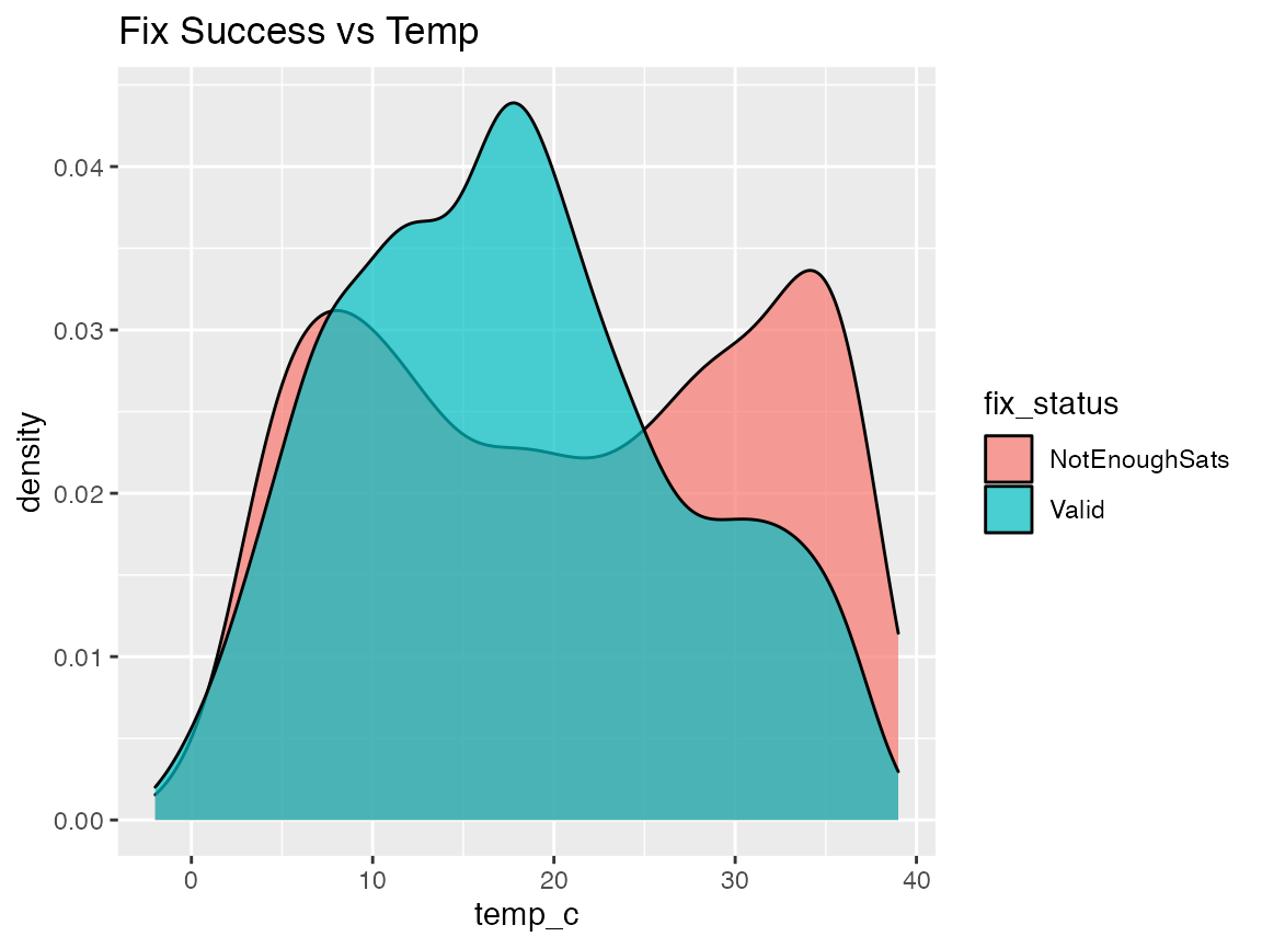
In this plot, we can see that the missed fixes are highly associated with the collar temperature. This indicates that the animals are resting in spots with poor satellite view. (Higher temperatures indicate the sensor is reading the animal’s body rather than the air.)
Given that caveat about bad data, missed fixes don’t actually have explicity spatial coordinates associated with them. So we will remove them for mapping.
library(mapview)
library(leaflet)
library(leaflet.providers)
get_animal_fixes(dsn) %>%
filter(fix_status == "Valid") %>%
mapview(zcol = "animal_id") ->
m
#> Reading layer `animal_fixes' from data source
#> `/Library/Frameworks/R.framework/Versions/4.1/Resources/library/beastr/db/telemetry.gpkg'
#> using driver `GPKG'
#> Simple feature collection with 4244 features and 12 fields (with 1990 geometries empty)
#> Geometry type: POINT
#> Dimension: XY
#> Bounding box: xmin: 251017.2 ymin: 4161726 xmax: 305421.4 ymax: 4227265
#> CRS: 32611
mYou may notice some outlying points. Obviously we have fixes with actual coordinates that still aren’t good. How can we remove these?
Filters
There are quite a few different measures of how bad a fix is. Some of these come with the data, and some we have to compute ourselves. The most reliable approach is to use multiple measures and filter the data based on thresholds. Picking these thresholds is somewhat mystical. Let’s take a look at some of them:
Dilution of Precision
Dilution of Precision (DOP) measures are calculated by the GPS receiver based on satellite precision. There are multiple variants. Common ones are horizontal and vertical. THe closer together the satellites are in the sky, the les
Lotek gives us horizontal dilution of precision (hdop). Let’s take a look at the distribution from our example dB:
get_animal_fixes(dsn) %>%
ggplot(aes(x = hdop)) +
geom_histogram(binwidth = 0.1) +
xlab("hdop, (log scale)") +
scale_x_log10()
#> Reading layer `animal_fixes' from data source
#> `/Library/Frameworks/R.framework/Versions/4.1/Resources/library/beastr/db/telemetry.gpkg'
#> using driver `GPKG'
#> Simple feature collection with 4244 features and 12 fields (with 1990 geometries empty)
#> Geometry type: POINT
#> Dimension: XY
#> Bounding box: xmin: 251017.2 ymin: 4161726 xmax: 305421.4 ymax: 4227265
#> CRS: 32611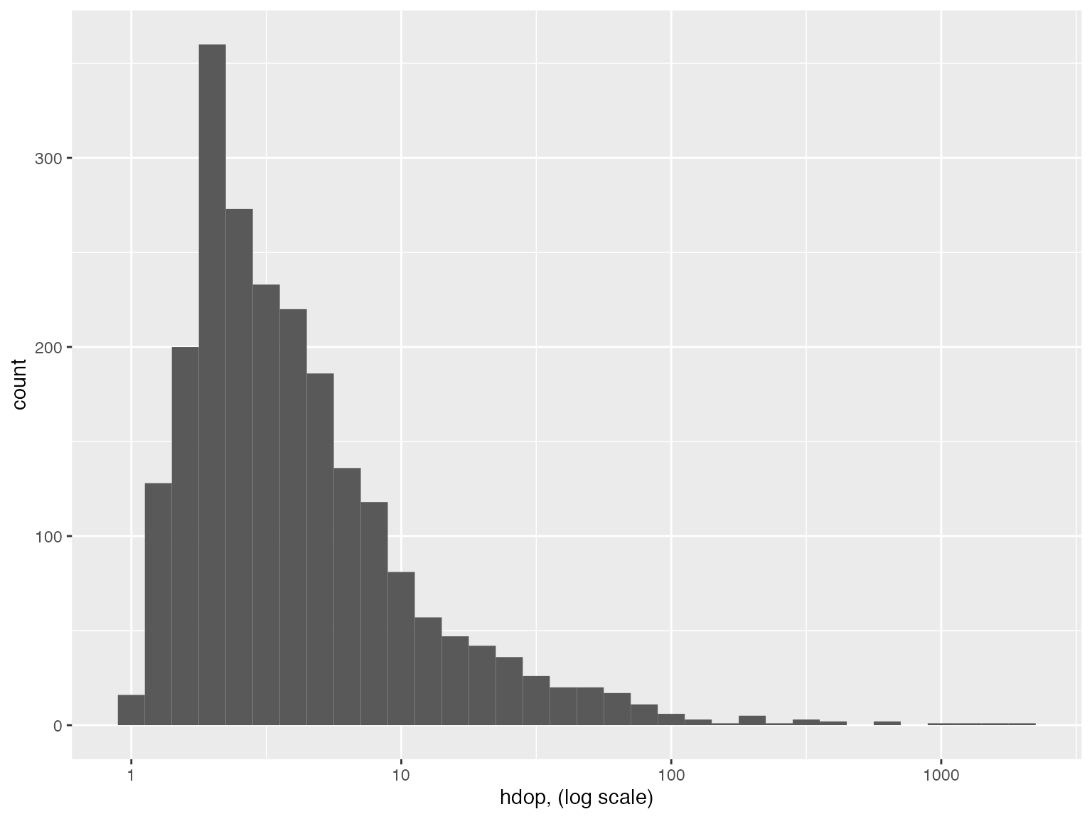
Here we can see that most of the HDOP values are under 10. The ones above 10 are likely to have a high error. We obviously don’t have a way to directly measure error for each of these points, but we can get an indication that hdop is associated with error by looking at displacement. In this case we can define displacement at the distance from the mean point. If high HDOP points tend to have high displacement, that’s a good indication that it is associated with error. Let’s take a look:
# load sf for spatial processing:
library(sf)
# calculate mean points per animal:
get_animal_fixes(dsn) %>%
group_by(animal_id) %>%
summarise(geom = sf::st_union(geom)) %>%
mutate(centroid = st_centroid(geom)) %>%
st_drop_geometry() ->
animal_centroids
#> Reading layer `animal_fixes' from data source
#> `/Library/Frameworks/R.framework/Versions/4.1/Resources/library/beastr/db/telemetry.gpkg'
#> using driver `GPKG'
#> Simple feature collection with 4244 features and 12 fields (with 1990 geometries empty)
#> Geometry type: POINT
#> Dimension: XY
#> Bounding box: xmin: 251017.2 ymin: 4161726 xmax: 305421.4 ymax: 4227265
#> CRS: 32611
# calculate displacement for each point
get_animal_fixes(dsn) %>%
filter(fix_status == "Valid") %>%
left_join(animal_centroids) %>%
mutate(disp = st_distance(geom, centroid, by_element = TRUE)) ->
fixes_w_displacement
#> Reading layer `animal_fixes' from data source
#> `/Library/Frameworks/R.framework/Versions/4.1/Resources/library/beastr/db/telemetry.gpkg'
#> using driver `GPKG'
#> Simple feature collection with 4244 features and 12 fields (with 1990 geometries empty)
#> Geometry type: POINT
#> Dimension: XY
#> Bounding box: xmin: 251017.2 ymin: 4161726 xmax: 305421.4 ymax: 4227265
#> CRS: 32611
# log scales:
fixes_w_displacement %>%
mutate(disp = as.numeric(disp)) %>%
ggplot(aes(x = disp, y = hdop)) +
geom_point(alpha = 0.5) +
scale_x_log10() +
scale_y_log10()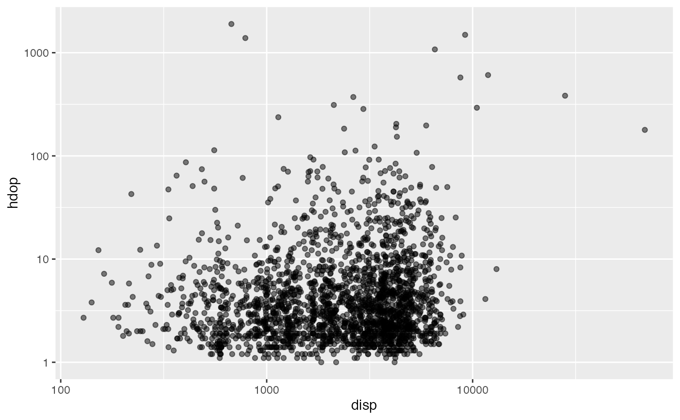
This is interesting because we see a natural boundary in displacement. This is at roughly 8km, so that makes sense for an animal (fisher in this case) staying within a typical home range. There are two distinct features of this plot to notice:
- Nearly all the points with displacement outside the typical homerange have high HDOP. These are almost certainly bad points. Points that we could probably tell are bad just from the map.
- There are, however, still many points within the typical displacements that have similarly high HDOP. These are the reason we need these data filters beyond just looking at the map and throwing away points that look absurd. These points might look normal on a map but are still probably bad.
From this plot, I would use the points in the upper right sector to pick an ad-hoc cutoff for HDOP. Probably ~100. It’s better to be conservative and not throw away too many points. That’s why we’ll apply multiple filters to narrow down other bad fixes. But first let’s see the data after filtering on HDOP:
get_animal_fixes(dsn) %>%
dplyr::filter(hdop < 100) %>%
mapview()
#> Reading layer `animal_fixes' from data source
#> `/Library/Frameworks/R.framework/Versions/4.1/Resources/library/beastr/db/telemetry.gpkg'
#> using driver `GPKG'
#> Simple feature collection with 4244 features and 12 fields (with 1990 geometries empty)
#> Geometry type: POINT
#> Dimension: XY
#> Bounding box: xmin: 251017.2 ymin: 4161726 xmax: 305421.4 ymax: 4227265
#> CRS: 32611Elevation Error
You are probably aware that GPS fixes locate the receiver in 3D space, and thus produce an elevation as well as coordinates. You are probably also aware that the vertical accuracy isn’t as good as the horizontal. We can use this to find more bad fixes that might still have a relatively low HDOP. If the point is good, the gps elevation should roughly agree with an external source, known as a Digital Elevation Model (DEM).
DEM files are very large, and the automated services to request DEM at specific points are quite slow for large datasets. So these filters rely on downloading external data not included in the package. There are many different DEM sources globally, but for this example we’ll use the USGS 1/3 Arc Second DEM. In this example all of our points are covered in one GeoTIFF. This GeoTIFF is converted into a stars object. If you have multiple files, they can be converted to a single stars, but that is outside of our scope. Please see stars
# Downloading a GeoTIFF for our area:
dem_url = "https://prd-tnm.s3.amazonaws.com/StagedProducts/Elevation/13/TIFF/historical/n38w120/USGS_13_n38w120_20210701.tif"
# change to your location!!
myDEM = system.file("myDem.tif", package="beastr")
# download file
download.file(dem_url, myDEM, method = "wget")Now that we’ve downloaded a DEM file, we can use get_elevation_dem to add a DEM elevation column to our fixes, or get_elevation_difference to directly add a column for the difference between the gps and dem elevations. Let’s take a look at the DEM elevation versus the GPS elevation:
fixes_w_displacement %>%
get_elevation_dem(dem_src = myDEM) %>%
ggplot(aes(x = elevation_dem, y = elevation_gps)) +
geom_point(aes(color = sqrt(as.numeric(disp)))) +
labs(color = "Root Displacement (m^0.5)") +
scale_color_viridis_c()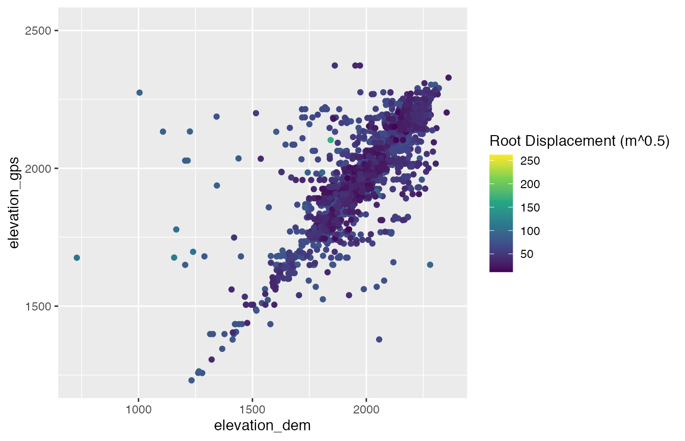
Here you can see that most of the time, these are pretty similar. Especially for low displacement points. But there are lots of points that differ by quite a bit. Something is fishy with these ones.
Let’s take a look versus displacement again:
fixes_w_displacement %>%
get_elevation_difference(dem_src = myDEM,
elev_field = elevation_gps) %>%
mutate(disp = as.numeric(disp)) %>%
ggplot(aes(x = disp, y = elevation_dif)) +
scale_x_log10() +
geom_point(alpha = 0.5) 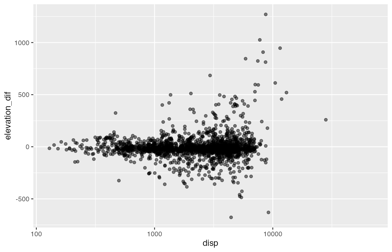
In this case, I’m not entirely sure what a good cutoff is, but let’s pick something and take a look at the points, this time filtering both HDOP and elevation difference:
get_animal_fixes(dsn) %>%
dplyr::filter(hdop < 100) %>%
get_elevation_difference(dem_src = myDEM, elev_field = elevation_gps) %>%
dplyr::filter(abs(elevation_dif) < 300) %>%
mapview(zcol = "animal_id")
#> Reading layer `animal_fixes' from data source
#> `/Library/Frameworks/R.framework/Versions/4.1/Resources/library/beastr/db/telemetry.gpkg'
#> using driver `GPKG'
#> Simple feature collection with 4244 features and 12 fields (with 1990 geometries empty)
#> Geometry type: POINT
#> Dimension: XY
#> Bounding box: xmin: 251017.2 ymin: 4161726 xmax: 305421.4 ymax: 4227265
#> CRS: 32611This is starting to look more like real data.